Solution
4 Row Pivot Table (Sorted) by Mark Kubiszyn
A brief outline of this Project and what is in the purchased file
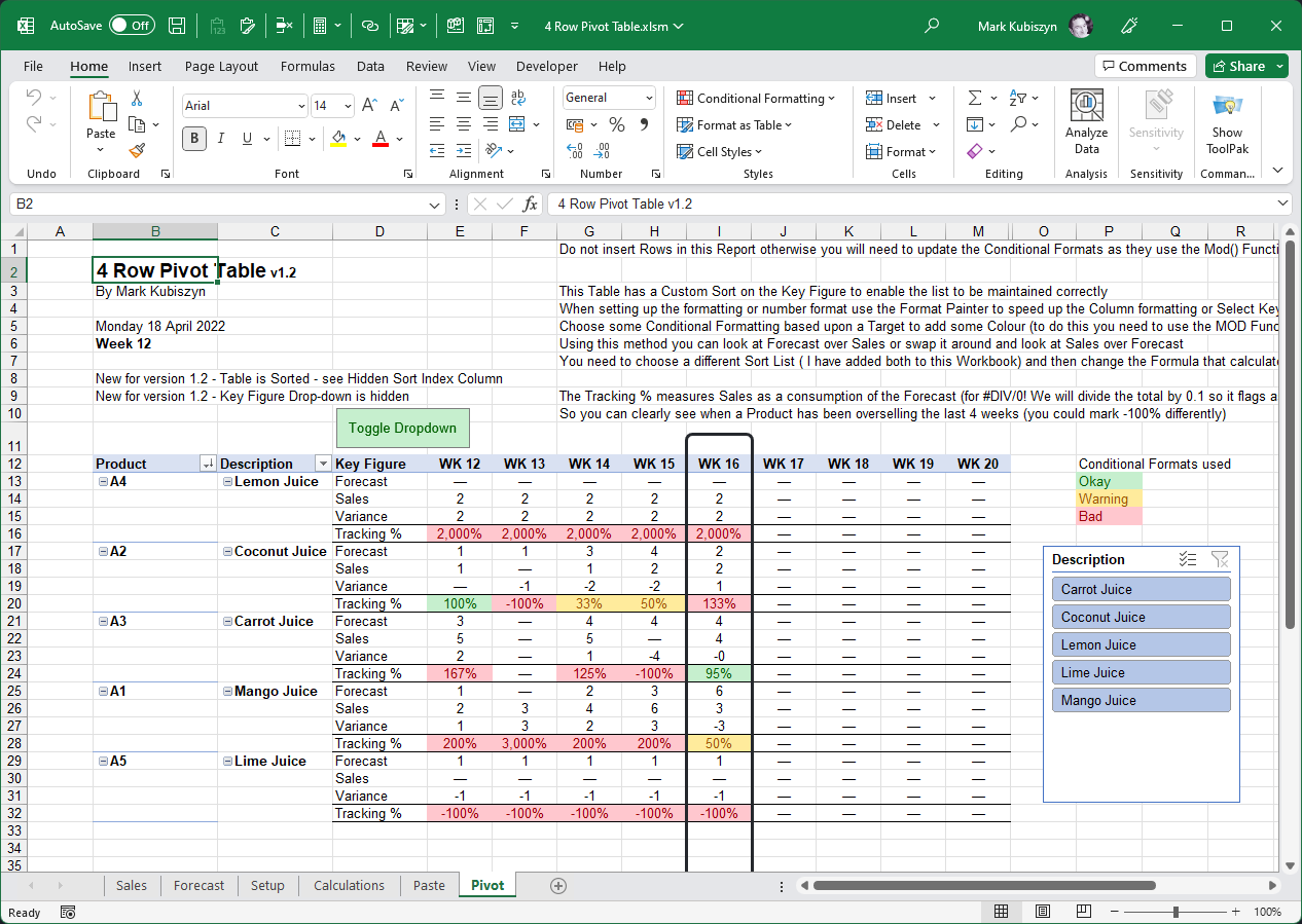
This Software will demonstrate a 'Solution' you can use to build a sorted, rolling 4 Row Pivot Table viewing Products with Sales, Forecast, Variance and Tracking % (4 Key Figures), from Sales and Forecast data using formula and a single Macro to update the Pivot Table week Fields. It allows you to keep your source data in Columns instead of transposing the weeks into Rows (a standard way of using rolling weeks is to have all of the weeks down the Rows and then to add a single 'Weeks' field into the Columns section). This method does not use any Calculated Items or Fields in the Pivot Table and allows you to Slice any data as long as it is on a 1-2-1 basis with the Products
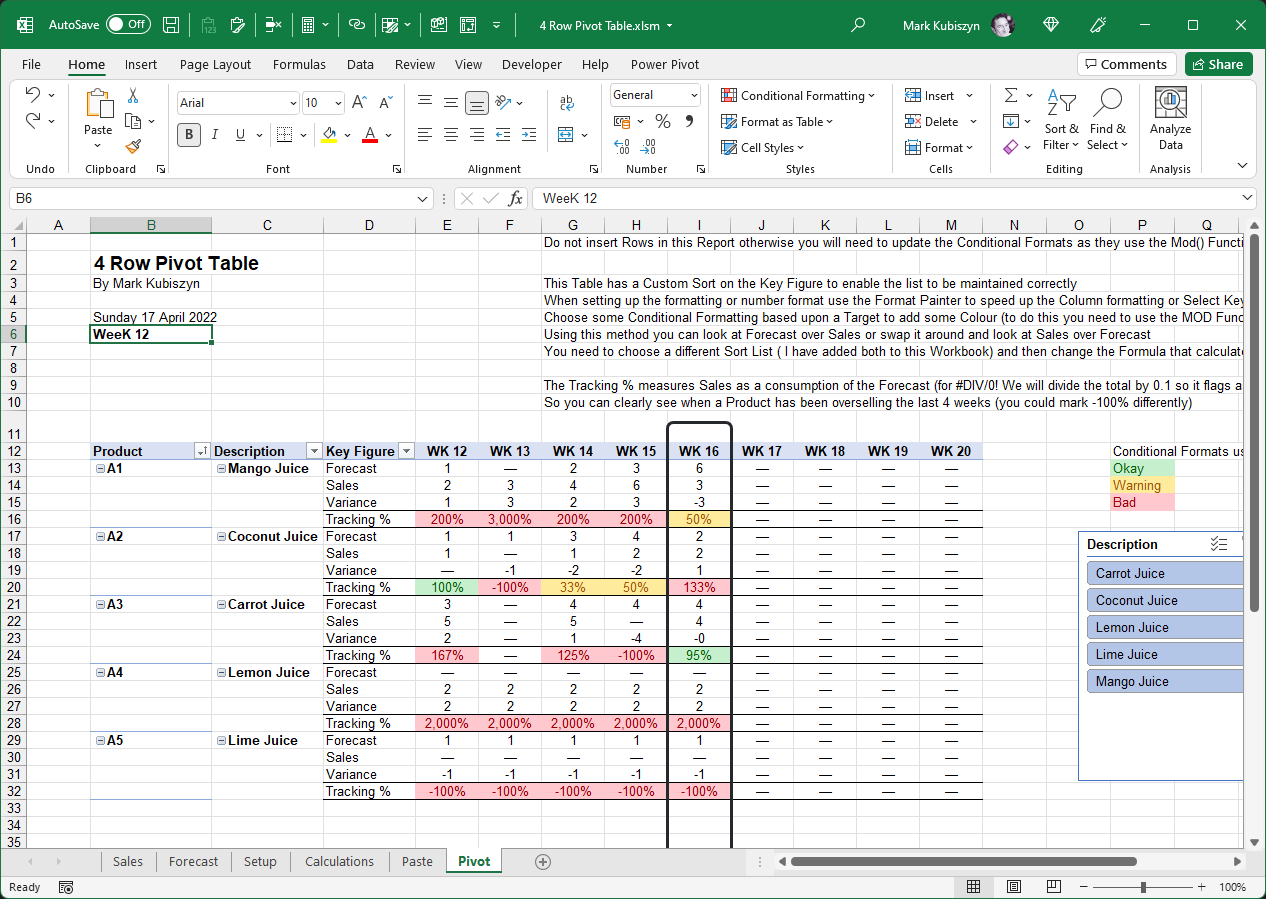
Each Product will have 4 Rows (Key Figures) in this order Forecast, Sales, Variance (the difference between the Forecast and the Sales) and the Tracking % (the consumption of the Sales against the Forecast as a percentage). The Conditional Formatting being measured for both +/- is Green (Okay) for within a 30% tolerance from 100%, Warning (Amber) for up to 70% tolerance from 100% and Red (Bad) for > 100% tolerance. Therefore, at a glance we can see that if a Product is all Green then the Sales are pretty much in line with the Forecast and if it is all Red then the Sales are most definitely not in line with the Forecast. The order of the 4 Key Figures can be changed along with the Formula for consumption ie. you could swap it around and do a consumption of the Forecast against the Sales
In version 1.2 I have added a Sort Index to enable you to Sort the 4-Row Pivot Table against how you are Tracking and Code to demonstrate toggling a Pivot Table Column Field Drop-down to Hide/Show it to the user
Prerequisites
- 32bit or 64bit Excel
- Basic Excel skills
- Windows PC · NOT a Mac!
- No support is provided for customization of this Software
Features
- A Multiple Row Pivot Table
- 4 Rows per Product detailing the Forecast, the Sales, a Variance and a Tracking %
- Demonstrates how to maintain and update a Rolling Window of Week Fields in a Pivot Table using source data in Weekly Columns as opposed to Rows and a small piece of VBA
- Conditional Formatting demonstrates how simple it is to use Colour as a visual aid to detail how the Sales is tracking against the Forecast. The Conditional Formatting being measured for both +/- is Green (Okay) for within a 30% tolerance from 100%, Warning (Amber) for up to 70% tolerance from 100% and Red (Bad) for > 100% tolerance
- Demonstrates how to workaround the #DIV/0! Error by dividing by 0.1 so Sales of 3 without a Forecast will be 3,000%, a Forecast of 3 without a Sales will be -100% and a Forecast of 3 and a Sales of 3 will be 100% - this allows us to employ the logic specified above for the Conditional Formatting
- Single Macro to Update the Pivot Table Weekly Column Fields as the Week numbers roll on throughout the Year
- Formula demonstrates how to build a unique list of Product from both of the Sales and Forecast Sheets
- Formula demonstrates how to build a repeated list of Products from the Setup Sheet and then generate the required 4 Rows of data per Product using the Key Figures alongside the Product Descriptions from both of the Sales and Forecast Sheet
- Demonstrates the use of a Drawing Object or Shape to use as a Marker to highlight the Current Week and how to Lock the Sheet for Drawing Objects including Slicers to prevent them from being moved around (Optional)
- Sort Index to enable you to Sort the 4-Row Pivot Table against how you are Tracking
- Code to Hide a specific Pivot Table Field Drop-down form the end user
Here is a Tracker Report I wrote using the METHODOLGY I use for the 4 Row Pivot Table but as a 3 Row Pivot Table showing you what is possible - PLEASE NOTE: this Report is NOT part of this Software and is NOT available for me to distribute!
How To
Step 1 - Gathering data
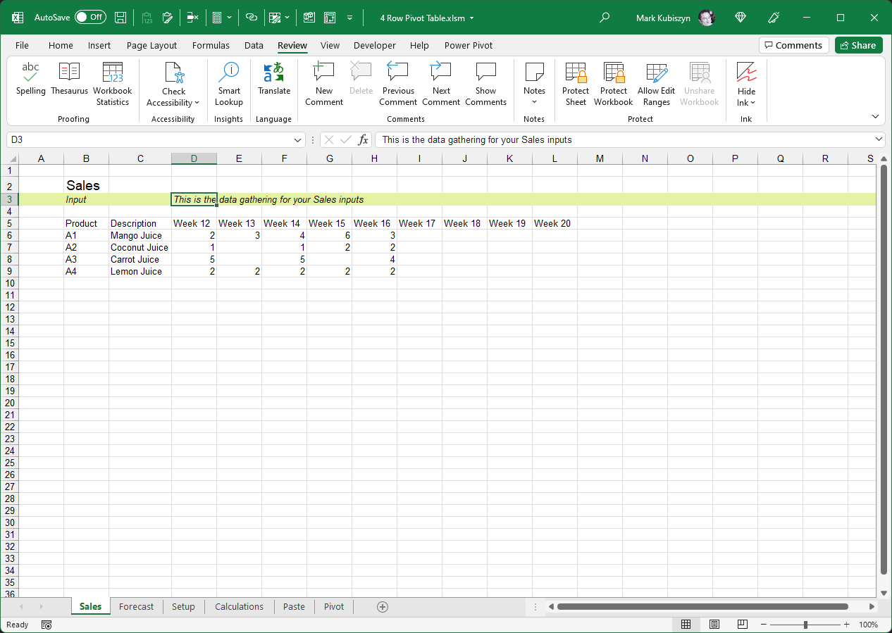
The first thing we need to do is to pull together both Sales and Forecast data for lets say 9 weeks, first 4 weeks past, current week and then the next 4 weeks
Here are my data inputs for the process - you will notice that the weekly Headers are slightly different for the Forecast than the Sales. This does not matter, just make sure that if you are changing these inputs for your own data, that you have Products, Product Descriptions and then 9 weeks of data going across the Columns. Ensure that your data is 1-2-1, meaning that each Product is unique and not for example Products by Depots. For my dummy data we will use Cartons of Juice. On the Sales Sheet I will have one Product, Lemon Juice that is not in the Forecast Sheet and on the Forecast Sheet I will have one Product Lime Juice that is not on the Sales Sheet. This will demonstrate the Formulas capability of picking up Products not featured on both Sheets. Notice that the Forecast may also be to 3 decimal places even though we will be Forecasting PC or each. This is also fairly typical in many systems when Forecasting through various aggregation levels. I have not increased the decimal places in the Pivot Table but you can easily do this if you want later on in the process. Week 16 is the current week:

Step 2 - The Setup
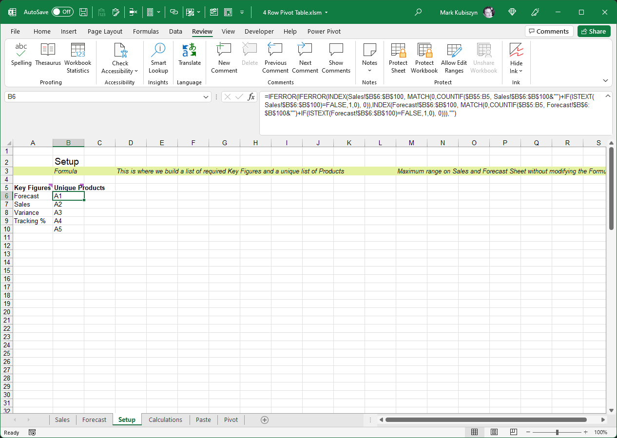
Next we will create the 4 Key Figures that we will use for the Pivot Table Rows. The values Forecast, Sales, Variance and Tracking % are entered in Cells "A6:A9". For brevity I entered them in the Sort order I want - this also makes it easier when writing the Formula (we can change the Sort order within the Pivot Table later on - I will show you how to do this). Now we will use a Formula to pull in the Unique Product Codes from both the Sales and Forecast Sheets. The Formula used will work for up to 100 Rows of data otherwise you will need to increase the 100 below to the new length of Rows down:
=IFERROR(IFERROR(INDEX(Sales!$B$6:$B$100, MATCH(0,COUNTIF($B$5:B5, Sales!$B$6:$B$100&"")+IF(ISTEXT(Sales!$B$6:$B$100)=FALSE,1,0), 0)),INDEX(Forecast!$B$6:$B$100, MATCH(0,COUNTIF($B$5:B5, Forecast!$B$6:$B$100&"")+IF(ISTEXT(Forecast!$B$6:$B$100)=FALSE,1,0), 0))),"")
Step 3 - The Calculations
Okay so the next step we have to do is to create the calculations that will become the input for our Pivot Table. This will include generating all of the required Product combinations together with each Key Figure and also looking up the Product Descriptions from both the Sales and Forecast Sheets. After we have done this, we will then create the Formula that pulls in the Sales and Forecast data and also performs the Variance and Tracking % calculations, for each Product, for each Key Figure, for each rolling week
The Formula for the first spawning of the Products, again for up to 100 Rows and to create 4 Rows per Product, is:
=IF(ROW()-ROW($B$6)+1>COUNTA(Setup!B$6:B$100)*COUNTA(Setup!A$6:A$100),"",INDEX(Setup!B$6:B$100,INT((ROW()-ROW($B$6))/COUNTA(Setup!A$6:A$100)+1)))
The next Formula to look up the Product Descriptions from both the Sales and the Forecast Sheets is (Please note: I have not tied this down to any Range - it will check the entire Columns on both Sheets):
=IFERROR(IFERROR(INDEX(Sales!C:C,MATCH($B6,Sales!B:B,0)),INDEX(Forecast!C:C,MATCH($B6,Forecast!B:B,0))),"")
Lastly we have the Formula that generates each Key Figure multiple times (this Formula check for a value in Cell "B6" and will output Blank if no values is found):
=IF($B6="","",IF(ROW()-ROW($D$6)+1>COUNTA(Setup!B$6:B$100)*COUNTA(Setup!A$6:A$100),"",INDEX(Setup!A$6:A$100,MOD(ROW()-ROW($D$6),COUNTA(Setup!A$6:A$100))+1)))
So now you can see the Results of the initial Calculations in the image below as well as the Formula that does the pulling of the Sales and Forecast data alongside the Variance and Tracking % calculations:
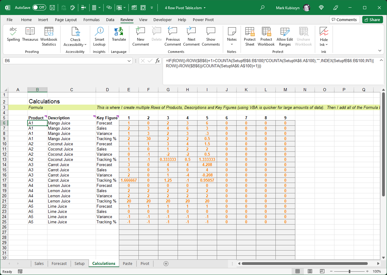
The Final Calculation is the one that we will drag across to derive our data for each week. This involves us making a check using =IF for each Key Figure and then doing 'some' calculation within the Formula accordingly - it looks like a lot of hard work, but it is fairly simple really. First of all we check for the Sales Key Figure. If we find it we then pull in any Sales data that matches the Product Code in Column B. We do the same for the Forecast Key Figure. If we find it we then pull in any Forecast data that matches the Product Code in Column B. Next we will check for the Variance Key Figure and if we find that we will do the Sales minus the Forecast. Lastly and a little more complex we check for the Tracking % and if we find that we switch on a number of possible outcomes. The Formula for this is "IFERROR(IF(AND(E3>0,E4<=0),-1,IF(AND(E4>0,E3<=0),E4/0.1,E4/E3)),0)". To explain if we have a Forecast without Sales then we output -1 (-100%), if we have a Sales without a Forecast we avoid the #DIV/0! Error by dividing the Sales by 0.1 ie. for 3 Sales and no Forecast we will get 3,000%, otherwise we will do the Sales divided by the Forecast ie. Sales of 3 with a Forecast of 6 will be 50% meaning that the Sales for that week were 50% of the overall Forecast for that week
=IFERROR(IF($D6="Sales",INDEX(Sales!D:D,MATCH($B6,Sales!$B:$B,0)),IF($D6="Forecast",INDEX(Forecast!D:D,MATCH($B6,Forecast!$B:$B,0)),IF($D6="Variance",E5-E4,IF($D6="Tracking %",IFERROR(IF(AND(E3>0,E4<=0),-1,IF(AND(E4>0,E3<=0),E4/0.1,E4/E3)),0),"")))),0)
Step 4 - Paste data
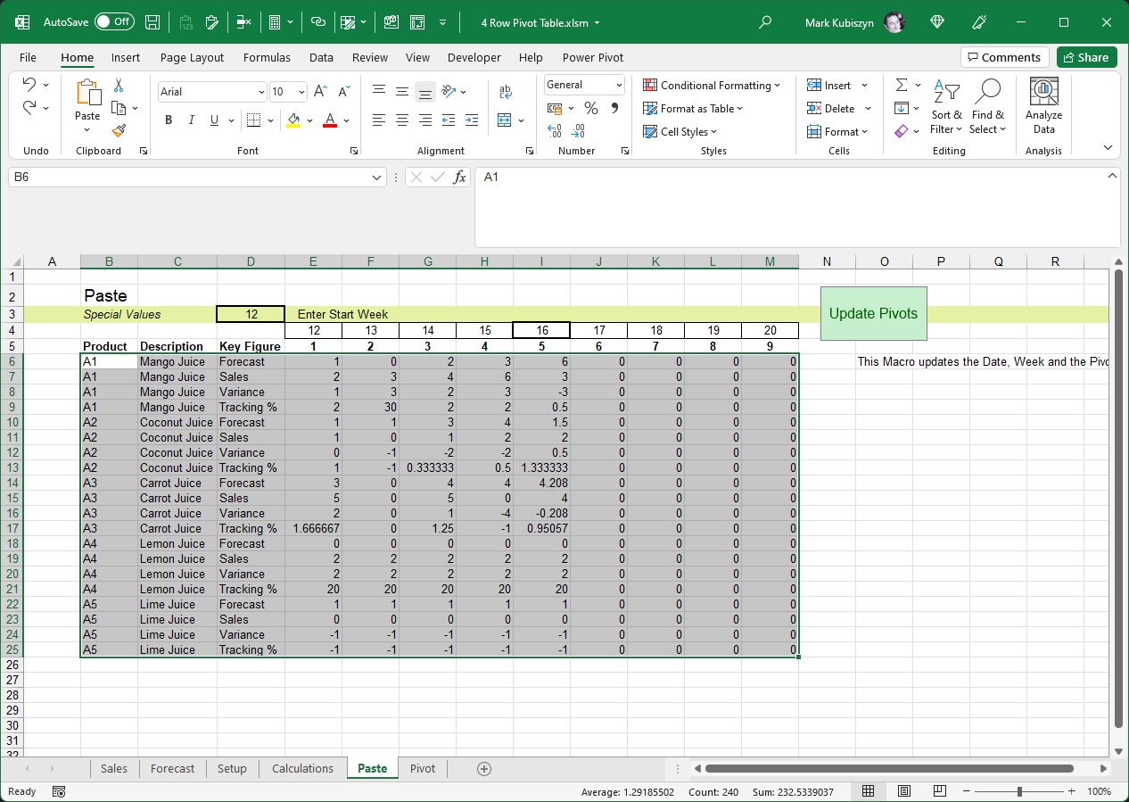
This is where we simply Copy & Paste the Calculations as Special Values underneath the headers. If we are Rolling the week ie. you have new data for a different week range, then enter a different Start Week in Cell "D3" - all of the weeks will change. Now run the Macro 'Update Pivots' to update and refresh the Pivot Table with the latest data and new Week Fields. A Named Range 'CurrentWeek' is used to capture the current week that is entered and a Named Range 'Headers' is used to capture the new Week Numbers
Step 5 - Pivot
This is the final 4 Row Pivot Table in all of its glory! The Sheet is Protected for Drawing Objects after the macro has been ran, meaning that you must Unprotect the Sheet before you can move the Slicer around or edit the marker. You can uncomment this in the Code if you wish so that nothing is locked when the Macro 'Update Pivots' is ran - go into the 'mdSubroutines' Code Module and comment out the Code below:
      .EnableSelection = xlNoRestrictions
      .Protect Contents:=False, UserInterfaceOnly:=True
Wrapping Up - So What Else Can You Do With This Technique?
Well, that's about it. Looking at the Pivot Table it is very Red indicating a majority oversell for most of the Products but then this is just dummy data! I like to also extend the Sales past the current week but I do not use the same Formula s I do not want to track Variance and Tracking % after the current week. I also like to show how the Current Week is tracking against a Daily target so I do this as an overview. Here is a Report I have built for the Company that I work for using the method outlined in this documentaion - it's pretty complex but very useful and includes a Sort algorithm to Sort my weekly Consumption as High/Low and last 2 week Variances as High/Low. I have had to blur confidential information and the Zoom is set at 70% but you can get a rough idea of what you can do. For this Tracker Report I only measured FCST, DEL and VAR, Forecast, Deliveries and Variance. I use a different Conditional Formatting for the Current Week to track versus a Daily target of 20% ie. Monday 20%, Tuesday 40% etc. I also added a Chart and a few more Pivot Tables to Track Category's in HL as opposed to PC (Each) which measures volume better as PC may show an incorrect percentage as you could have some Products like WINE selling thousands of Bottles if the Base Unit of Measure is Bottle, whereas HL will convert these thousands of Bottles into a more precise volume measurement

Magic Formula
Okay so it isn't really magic but lets take a look at the formula that will do the work of pulling in the values for our multiple Key Figures. As this formula may get quite large it is best to only use say4 or 5 Key Figures. You can use the =CHOOSE() function or =IF() for your decision switches. For my example I will use =IF() but space it out so when you are reading the Formula it kind of makes more sense. Once we have finished we will wrap all of the Formula in an =IFERROR(). Hopefully this will make things a little easier once you have grasped the concept and are creating your own multiple Row Pivot Tables
Please note: this Fomula may differ from the one included in this Software but will be broken down so that it is both easier to understand and easier to create for new Pivot Table Source data. In this example our Product Code is in Cell "B6" down Column B and each Key Figure is in Cell "D6" down Column D
Okay so the order that you perform the calculations using the Formula is irrelevant other than for brevity but lets take each Key Figure in turn. We will start with the Forecast Key Figure. Now if the Key Figure "Forecast" is found in Cell D6, the Formula below will bring back the Forecast in Column D on the Forecast Sheet for the Product in Cell "B6" down Column B matching the Product in the Forecast Sheet in Column B using a simple Index(), Match() combination (notice I have left a "NEXT KF" as the result if the Key Figure is not "Forecast" and I indented the "NEXT KF" by 2 spaces):
=IF($D6="Forecast",INDEX(Forecast!D:D,MATCH($B6,Forecast!$B:$B,0)),
  "NEXT KF"
)
Next we will do the Sales Key Figure. We will do exactly the same calculation to find the Sale in Column D on the Sales Sheet. We will place this part of the Formula ontop of the "NEXT KF" and then add 1 more end Bracket to the Formula like this (notice I have now Indented the middle part by 4 spaces so it is easier to read so the first =IF() does the Forecast and the second =IF() does the Sales):
=IF($D6="Forecast",INDEX(Forecast!D:D,MATCH($B6,Forecast!$B:$B,0)),
    IF($D6="Sales",INDEX(Sales!D:D,MATCH($B6,Sales!$B:$B,0)),
      "NEXT KF"
))
Please note: the next 2 parts are Formula based upon the results of the previous 2 Formula, the Forecast and the Sales. Okay, the next part of the Formula is a simple calculation between the Sales and Forecast ie. Sales - Forecast. For this Formula you will need to refer the Cells for the Calculation from above even though they may not be the final Cells you want to perform the Calculation on - this is so, that once you come across the "Variance" Key Figure the Formula will work correctly. Again I place this part of the Formula ontop of the "NEXT KF" like this (notice a further Indent of 2 spaces and another extra Bracket; isn't this fairly simple to do and read?):
=IF($D6="Forecast",INDEX(Forecast!D:D,MATCH($B6,Forecast!$B:$B,0)),
    IF($D6="Sales",INDEX(Sales!D:D,MATCH($B6,Sales!$B:$B,0)),
      IF($D6="Variance",E5-E4,
        "NEXT KF"
)))
Lastly I do the final Calculation for the Tracking % Key Figure. This is fairly complex and may differ to what you want to do, but for this example I do some switching within the Formula itself and also wrap this part of the Formula in IFERROR() to output zero (0) for errors. I check for whether there is a Forecast and no Sales so I want to output -100% or -1. I check for whether there is Sales but no Forecast and if this is TRUE I divide the Forecast by 0.1 (this avoids a DIV by zero error) and if this is FALSE I divide the Sales by the Forecast to give me the consumption of the Sales over the Forecast ie. Forecast = 6, Sales = 3 will equal 50% or 0.5. Here is my Tracking % Formula and once again I place this part of the Formula ontop of the "NEXT KF" like this (notice that again I add the "NEXT KF" and I indent by 2 more spaces)
=IF($D6="Forecast",INDEX(Forecast!D:D,MATCH($B6,Forecast!$B:$B,0)),
    IF($D6="Sales",INDEX(Sales!D:D,MATCH($B6,Sales!$B:$B,0)),
      IF($D6="Variance",E5-E4,
        IF($D6="Tracking %",IFERROR(IF(AND(E3>0,E4<=0),-1,IF(AND(E4>0,E3<=0),E4/0.1,E4/E3)),0),
          "NEXT KF"
))))
So now we are almost finished. If you needed more Formula for more Key Figures then you can continue this method. We don't so we now make 2 final changes to the Formula. First of all we replace the "NEXT KF" with "" (a pair of quotations) and then lastly we wrap it all up in an =IFERROR() outputting a zero (0) on any errors and tidy up the spacing to look like this - sweet eh? ;):
=IFERROR(
  IF($D6="Forecast",INDEX(Forecast!D:D,MATCH($B6,Forecast!$B:$B,0)),
    IF($D6="Sales",INDEX(Sales!D:D,MATCH($B6,Sales!$B:$B,0)),
      IF($D6="Variance",E5-E4,
        IF($D6="Tracking %",IFERROR(IF(AND(E3>0,E4<=0),-1,IF(AND(E4>0,E3<=0),E4/0.1,E4/E3)),0),
          ""
  )))),
0)
Hiding a Drop-down on a Pivot Field
When creating these types of Pivot Tables, you would normally not want a user to be able to Filter or Sort by the Key Figure Field. So to hide a Drop-down on a Pivot Field you can employ the following Code (add the Code to a Standard Code Module and then change the Pivot Table to your Pivot Table Name and the Field to your Field Name):
' use this to hide/disable a Drop-down in a Pivot Table by the Field Name
Private Sub DisableKeyFigureSelection()
   Dim pt As PivotTable
   Dim pf As PivotField
   On Error Resume Next
   Set pt = ActiveSheet.PivotTables("PivotTable1")
   For Each pf In pt.PivotFields
      If pf.Name = "Key Figure" Then pf.EnableItemSelection = False
   Next pf
   On Error GoTo 0
End Sub
Sorting the Pivot Table
To enable the Pivot Table to be Sorted you first need to add a 'Sort Index' Column at the end of the Data Source for the Pivot Table and a Formula that will capture how you are Tracking against the current week like this (see the Paste Sheet, Cell "N6"):
=IF($D6="Tracking %",$I6,N7)
Support
Support is 100% optional and I provide it for your convenience, so please be patient, polite and respectful
Support for my Software
- Responding to questions or problems regarding the Software and its features
- Fixing valid (replicated) bugs and reported issues for the VERSION I HAVE WRITTEN
Software support does not include
- Customization and installation services
- Support for third party software or ANY kind of development whatsoever
Before seeking support
- Make sure your question is a valid Software Issue and not a customization request
- Make sure you have read through the FAQ's, online documentation and any related video guides before asking support on how to accomplish a task
- Ensure that you access to the VBOM is allowed and that Macros can run in Excel
- Make sure to provide 'proof of purchase' and state the name / version of the Software that you are having issues with when requesting support by Email or via Facebook
How to get Support
Contact Mark Kubiszyn on the Email address provided when you purchased the Software, including the Order Number
Remember to be patient, if there has been an issue with your download, Mark will always respond within 48 hours and will Email you the File directly if neccessary. For other issues the response time may be considerably longer and I may choose to respond to specific questions only (as is my right), depending on what has been asked
Changelog
You can find the version history below - the latest Version including a description of any changes made is always shown first:
15.09.2022 - (Version 1.2) Released
Added in a Sort Index to enable you to Sort the 4-Row Pivot Table
Added in Code to demonstrate toggling a Pivot Table Column Field Drop-down to Hide/Show it to the user
24.04.2022 - (Version 1.1) Released
General release of the 4 Row Pivot Table